A short introduction to R
Current Versions of R and RStudio
Your R version should be 3.6.1.
Check this with
getRversion()## [1] '3.6.2'If this is not true, please go to https://cran.r-project.org/ and download Version 3.6.1.
The current version of RStudio should be Version 1.2.5001. Check here: https://rstudio.com/products/rstudio/download/ for current version.
General usage
Starting and closing RStudio, and the general usage of objects in your R workspace.
Whenever you start RStudio, a new session of R is started. RStudio has several panels, and one of them, called Console, is your connection to R in which you can execute R code directly. You can for example use the R console as a calculator e.g. by typing
1 + 2## [1] 3this will show you the calculated result immediatly.
However, as using numerical or string/character (e.g. “hello R world”) values directly has its limitations a central feature of most if not all programming languages including R are so called valiables. A variable is an entity that has a name and a value. E.g. you can create an object of the name x that has the value 17 by typing
x = 17If you now type the name of the object
x## [1] 17you will get the object’s value (in this case 17).
The reason for this is that R has temporarily saved this object (and its value) into R’s workspace.
We can check this by listing all objects by using the ls() function:
ls()## [1] "x"and we will see all the objects that are temporarily in our workspace. Alternatively, RStudio also provieds the Environment tab in on e of its panes.
When it comes the time to close RStudio (and therefore our R session), R will check whether the current workspace is empty or not (or: not changed or changed). If it is not empty (or if it is changed), we will be asked whether we wanted to save our current workspace (Save workspace image to ~/.RData?).
If we click on No, our object a will be lost, and we would have to recreate it in the next session (at least in the unlikely case that we will need it again).
If we click on Yes, however, the workspace image will be saved (into a file of the name ‘.RData’); this file will be loaded whenever we will start an R session in the future. If we then create new objects and continue with saving our workspace to the file ‘.RData’, this file will grow; after some time, this may lead to a longer loading time whenever we try to start R, and we will probably get confused about objects that we had created a long time ago, and that are no longer needed.
Therefore, in most cases we will not want to save all objects in our workspace to the file ‘.RData’. We advise you to click on No whenever you will be asked whether you wanted to save your workspace. Instead, you can save certain objects in your workspace permanently into an RData-file with a name given by you, and reload these objects whenever (and only then) you are in need of them (see below). The only exception to our advice is given whenever you really want to save a couple of objects that you will need in any future session. In our case, this is true for a few objects containing paths, from which we will be able to load speech and other data.
Before we create these path-objects and save them permanently, we should clean up our workspace. This can be done by simply closing RStudio and by answering No.
By the way, we could close the R session and RStudio also by typing
q()Data import and export
We will have to import data from an external source and to save data (including speech data) on our own computer. In order to to do so, the first step will be to create a folder on your computer. Please create (in your file browser) a folder called myEMURdata somewhere on your computer. Now find the correct path to this folder. This could be something like /Users/reubold/myEMURdata.
Now reopen RStudio and create an object in R called course_data_dir that contains your path (must be within " "):
course_data_dir = "/homes/<username>/myEMURdata" # substitute <username> with your name (linux) or adapt to path on your system entirely The varibale with your path can be listed as follows
ls()## [1] "course_data_dir"and you can call your path by
course_data_dir## [1] "./myEMURdata"However, this is just a confirmation of the existence of an object and its value. In order to confirm that the directory really exists, you need to type
dir.exists(course_data_dir)## [1] TRUEIt is also possible to specify a called URL (Uniform Resource Locator) to specify the location of a resource (e.g. data). In this case, the function dir.exists() will fail.
For loading data, we will use a specific URL (already known to those users familiar with the statistics seminar)
course_data_url = "http://www.phonetik.uni-muenchen.de/~jmh/lehre/Rdf"
dir.exists(course_data_url)
## [1] FALSEAlthough dir.exists() fails, this URL is correct! It is worth noting that in R it is possible to check if a URL is valid/exists or not (e.g. httr::url_ok() or RCurl::url.exists()) but we have not covered packages the use of packages yet.
Now, you should close RStudio and save the current workspace into ~/.RData by simply clicking on Yes (only this one time!). course_data_dir and course_data_url should then be available whenever you open a new R session.
Now, restart RStudio, and verify the existence of course_data_dir and course_data_url
ls()## [1] "course_data_dir" "course_data_url"From now on, we are able to load data from both paths, and to save data to course_data_dir (course_data_url is read-only).
ai = read.table(file.path(course_data_url, "ai.txt")) # Note: it is actually preferable to use the readr package for tabular data read/write (for simplicity we are using R's own read.table; more about packages to follow)An explanation:
file.path(course_data_url, "ai.txt") # creates a new path, by adding '/' to "course_data_url" and then concatenating this to "ai.txt"## [1] "http://www.phonetik.uni-muenchen.de/~jmh/lehre/Rdf/ai.txt"read.table() reads a table (related commands loading data see below…) from a file and creates a so-called data.frame
You can now work with this table (in its present format ‘data.frame’) in R
ai## F1 Kiefer Lippe
## 1 773 -25.47651 -24.59616
## 2 287 -27.02695 -26.44491
## 3 1006 -27.24509 -27.59161
## 4 814 -26.05803 -27.17365
## 5 814 -26.15489 -25.93095
## 6 806 -26.37281 -24.44872
## 7 938 -27.35341 -27.22650
## 8 1005 -27.98772 -28.26871
## 9 964 -26.27536 -27.05215
## 10 931 -26.09928 -26.54016
## 11 926 -26.40012 -26.83834
## 12 556 -25.73544 -27.21908
## 13 707 -25.84109 -23.44627
## 14 829 -26.37598 -25.23304
## 15 927 -27.47505 -27.64328
## 16 951 -26.68685 -25.63057
## 17 775 -25.79928 -23.68594
## 18 938 -27.18105 -25.28667
## 19 986 -27.75178 -27.70719
## 20 888 -25.99100 -26.84534
## 21 988 -26.27380 -28.26909
## 22 650 -26.50057 -24.31192
## 23 1026 -27.10303 -24.64248
## 24 992 -28.41081 -28.30641
## 25 896 -26.57372 -25.69383and/or you can now save this object as a table-like txt-document via
readr::write_tsv(ai, file.path(course_data_dir, "my_ai.txt"))Please confirm externally the existence of a file calles ‘my_ai.txt’ in your personal folder course_data_dir!
Download of (speech) data
Often we will have to download (speech) data to then be able to further process it in R. Although this it is possible to preform these types of procedures in R directly it is usually much simpler to use your operating system and a browser. Therefore, simply click directly onto the link in the present html document in order to download (speech) data. E.g., try to download testsample.zip!
Please save the zip-file ‘testsample.zip’ in your personal directory given in course_data_dir. Unzip it, and confirm the existence of the folder ‘testsample’ containing two sub-folders, ‘german’ and ‘nze’ (each of these sub-folders contains wav and txt files). We will work with this data soon.
Types of variables/objects
You can create an object and assign a value to it using either ‘=’ or ‘<-’
# numerical objects
a = 3
b <- 4

# objects containing characters and/or character strings need " "
c = "something"

# in R all objects of these basic types can contain more than one entity; assignment has then to be done with the combine function 'c()':

d = c(3, 4)
e = c("three", "four")

# Objects can also be tables; these can be of type 'matrix' (= all elements are of the same type, e.g. numeric)
# or of the type 'data.frame' (= its elements may have mixed types; columns have column names ...), e.g.
# Note: there are also other types of objects in R e.g. lists
ai
## F1 Kiefer Lippe
## 1 773 -25.47651 -24.59616
## 2 287 -27.02695 -26.44491
## 3 1006 -27.24509 -27.59161
## 4 814 -26.05803 -27.17365
## 5 814 -26.15489 -25.93095
## 6 806 -26.37281 -24.44872
## 7 938 -27.35341 -27.22650
## 8 1005 -27.98772 -28.26871
## 9 964 -26.27536 -27.05215
## 10 931 -26.09928 -26.54016
## 11 926 -26.40012 -26.83834
## 12 556 -25.73544 -27.21908
## 13 707 -25.84109 -23.44627
## 14 829 -26.37598 -25.23304
## 15 927 -27.47505 -27.64328
## 16 951 -26.68685 -25.63057
## 17 775 -25.79928 -23.68594
## 18 938 -27.18105 -25.28667
## 19 986 -27.75178 -27.70719
## 20 888 -25.99100 -26.84534
## 21 988 -26.27380 -28.26909
## 22 650 -26.50057 -24.31192
## 23 1026 -27.10303 -24.64248
## 24 992 -28.41081 -28.30641
## 25 896 -26.57372 -25.69383To see an object’s value(s), simply type its name
a## [1] 3To see an object’s type, do
is(a)## [1] "numeric" "vector"Create new objects with the same contents:
x = y = z = 4It is worth noting that objects can easily become overridden; you need to be careful, as you will get no warning:
y = 4
y
## [1] 4y = "phonetics"
y## [1] "phonetics"Saving objects in R’s workspace
Save objects with save(). You need to define the objects to be saved via list = and path and file name via file =
To save everything in your workspace, you can use the function ls(), which lists all objects in your workspace. However, this is identical to closing RStudio and replying Yesto the question Save workspace image to ~/.RData? [y/n/c]::
save(list = ls(), file = file.path(course_data_dir, "objects.RData"))
save(list = ls(), file = file.path(course_data_dir, "objects"))
The file name (here: ‘objects’) is up to you! You have now created two files in your folder, one without any extension, one with the extension ‘.RData’. Both have identical file sizes, and both can be loaded into R with the function load() or attach(). The advantage of extension ‘.RData’ is that you can load its contents into R via a double click on the file (corresponds to load()) and it also indicates to the user what type of data is contained within that file (same as other extensions .docx or .wav).
attach() or load() objects
Close RStudio/R (do NOT save the workspace), and restart it again, and then:
attach(file.path(course_data_dir, "objects"))## The following objects are masked _by_ .GlobalEnv:
##
## ai, course_data_dir, course_data_urla## [1] 3b## [1] 4c## [1] "something"I.e., you can call the objects’ contents; however, the objects will not be listed by ls()
ls()## [1] "ai" "course_data_dir" "course_data_url"Attached files containing objects can, however, be seen by typing
search()## [1] ".GlobalEnv" "file:./myEMURdata/objects"
## [3] "package:emuR" "package:stats"
## [5] "package:graphics" "package:grDevices"
## [7] "package:utils" "package:datasets"
## [9] "package:methods" "Autoloads"
## [11] "package:base"detach() can remove certain entities (here: the second entry = path to the file) in the search-path:
detach(2)
search()
## [1] ".GlobalEnv" "package:emuR" "package:stats"
## [4] "package:graphics" "package:grDevices" "package:utils"
## [7] "package:datasets" "package:methods" "Autoloads"
## [10] "package:base"Objects’ contents like that of x are now no longer available:
x## Error in eval(expr, envir, enclos): Objekt 'x' nicht gefundenAlternatively: load() ‘objects’ or ‘objects.RData’ or simply double click on ‘objects.RData’
load(file.path(course_data_dir, "objects.RData"))
ls()
## [1] "a" "ai" "b" "c"
## [5] "course_data_dir" "course_data_url" "d" "e"
## [9] "x" "y" "z"The saved objects are now in your workspace. In order to remove certain objects, use rm(), e.g.:
rm(list=c("x","y","z"))
ls()
## [1] "a" "ai" "b" "c"
## [5] "course_data_dir" "course_data_url" "d" "e"In order to remove all objects, you could do:
rm(list=ls())
However, this would also delete course_data_dir and course_data_url; so you should preferably simply close RStudio (again: without saving the workspace!) and reopen it.
Packages
Functions in R have a name, followed by (...); ... stands for object names and/or certain parameters; most function names are more or less self explanatory (save(), load(), read.table() and the like): some of them need a bit more of a good guess, e.g. in order to list objects, use the function ls():
ls()## [1] "ai" "course_data_dir" "course_data_url"R comes with many functions (see e.g. http://cran.r-project.org/doc/contrib/Short-refcard.pdf for an overview over the most common ones).
However, many functions that we will need are not available in base R, especially none for working with speech databases, of course. However, many more specialized functions have been made available by developers of so-called packages. To make these functions available to us, we need to install the corresponding packages.
In RStudio:
Tools–>Install Packages
or install.packages("packagename"); e.g. we will need “emuR” for speech database creation an analysis, “tidyverse” for the manipulation and plotting of data (the tidyverse defines a specific group of R packages that are often used together incl. but not limited to ggplot and dplyr; see https://www.tidyverse.org/):
install.packages("emuR")
install.packages("tidyverse")
After the installation process (which might take a while), you still have to attach the functions to R’s search path; e.g. function ggplot() and geom_boxplot() will not be available, unless you attached it to the search path by using library(ggplot2)
ggplot(data = ai, aes(x = "", y = F1)) +
  geom_boxplot()
## Error in ggplot(data = ai, aes(x = "", y = F1)): konnte Funktion "ggplot" nicht findenlibrary(ggplot2)
ggplot(data = ai, aes(x = "", y = F1)) +
geom_boxplot()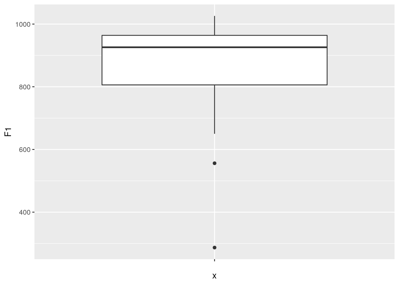
Use search() and detach() in order to remove function names of certain packages from R’s search path:
search()## [1] ".GlobalEnv" "package:ggplot2" "package:emuR"
## [4] "package:stats" "package:graphics" "package:grDevices"
## [7] "package:utils" "package:datasets" "package:methods"
## [10] "Autoloads" "package:base"ggplot2 is listed as number 2, so remove it by
detach(2)
geom_boxplot()
## Error in geom_boxplot(): konnte Funktion "geom_boxplot" nicht findenThis may be necessary, whenever R tries to apply the ‘wrong’ function; this may happen whenever you have more than one package loaded, and functions of these packages accidentally share the same name.
Alternatively, you could also try to call the function by adding the correct package’s name with package::function, like e.g.
ggplot2::geom_boxplot()## geom_boxplot: outlier.colour = NULL, outlier.fill = NULL, outlier.shape = 19, outlier.size = 1.5, outlier.stroke = 0.5, outlier.alpha = NULL, notch = FALSE, notchwidth = 0.5, varwidth = FALSE, na.rm = FALSE
## stat_boxplot: na.rm = FALSE
## position_dodge2Another advantage of this procedure is - as you can see above - that the function will be available although you haven’t loaded the package (ggplot2 is NOT in the R search path right now…)
Help
General Introduction
See ‘An Introduction to R’ in:
help.start()Help about certain functions
You want to know more about a certain function, like pnorm()?
help(pnorm)
# oder
?pnorm

example(density)

apropos("spline")

help.search("norm")
Of course, you need to know the function’s name in order to call for help. In order to get a list of all functions of a package, type library(help=PACKAGE), e.g.
library(help=emuR)A document will open; go to ‘Index’ and find a list of names of functions (and possibly objects) and a short description of what the function does (or what the object contains). For a closer examination, copy a function’s name and paste it into one of ?FUNCTIONNAME or help(FUNCTIONNAME) or help("FUNCTIONNAME")
You could also use the packages’ reference manuals, e.g.
https://cran.r-project.org/web/packages/emuR/emuR.pdf
Vignettes
Another possibility which is closer to an in-depth introduction (but possibly missing some of the package’s functions) is given in some packages by the so-called vignettes. They usually deliver an exemplary workflow (and therefore usually explain more than one function at once); vignettes are delivered in html or pdf format, and can be viewed externally or in RStudio’s Viewer; in order to look for all available vignettes (of all packages), call
vignette()Read these vignettes by typing vignette("VIGNETTENAME"), e.g.
vignette("dplyr")VIGNETTENAMEs are not necessarily identical to the name of the package.
The EMU-SDMS-Manual
The best way to get help about emuR is to be found here: https://ips-lmu.github.io/The-EMU-SDMS-Manual/index.html
Comments R Scripts (.R) and R Markdown (.Rmd) files
Punching in R code directly into the console has severe limitations. For reproducibility and other reasons it is highly advisable to save your R code in text files containing said code. The convention is to use the extension .R for these types of files to mark that they contain R code. Within these files there are only two types of lines:
the first of which (lines beginning with #) are simply ignored by R and are considered as comments. The later, are considered to be R code and are executed:
These .R files are still by far the most common way to store R code. However, in recent years a new format has become more and more popular. The R Markdown, albeit being an extension to the pre-existing Markdown, is a so called markup language (same as HTML -> Hypertext Markup Language). However, it is so simple that the inventors decided to call it Markdown. It basically allows the user to simply structure their texts using characters that have special meanings e.g. the # character:
or the
-character:see https://rmarkdown.rstudio.com/lesson-1.html for a detailed introduction.
The things that differentiates R Markdown from regular Markdown are R code blocks that contain R code that can be executed or not. These code blocks begin with the following chain of characters ```{r} and end with ```. The code contained within these symbols is interpreted as R code. The advantage of these files is that they can easily translated in various different widely used formats (HTML, PDF, Word, …) for example the file that you are currently looking at was written in R Markdown and then translated to HTML using R packages. R Markdown files can easily be created in R Studio:
File -> New File -> R Markdown....So when should I use .R vs .Rmd`: A good rule of thumb is: if your file contains way more comments than actual R code it might be worth considering writing it in R Markdown.